A simple explanation of the Inception Score
The Inception score (IS) is a popular metric for judging the image outputs of Generative Adversarial Networks (GANs). A GAN is a network that learns how to generate (hopefully realistic looking) new unique images similar to its training data. Most papers about GANs use the IS to show their improvement versus the prior art:
“…our models (BigGANs) achieve an Inception Score (IS) of 166.3 and Frećhet Inception Distance (FID) of 9.6, improving over the previous best IS of 52.52 and FID of 18.65.” — From Large Scale GAN Training for High Fidelity Natural Image Synthesis
I found a lot of the online explanations of the Inception Score unnecessarily hard to follow, cloaking its workings in mathematical jargon. Hopefully this one is easier to follow :)

What is the Inception score?
The IS takes a list of images and returns a single floating point number, the score.
The score is a measure of how realistic a GAN’s output is. In the words of its authors, “we find [the IS] to correlate well with human evaluation [of image quality]”. It is an automatic alternative to having humans grade the quality of images.
The score measures two things simultaneously:
- The images have variety (e.g. each image is a different breed of dog)
- Each image distinctly looks like something (e.g. one image is clearly a Poodle, the next a great example of a French Bulldog)
If both things are true, the score will be high. If either or both are false, the score will be low.
A higher score is better. It means your GAN can generate many different distinct images.
The lowest score possible is zero. Mathematically the highest possible score is infinity, although in practice there will probably emerge a non-infinite ceiling¹.
The IS has proven itself useful and popular, although it has limitations (covered in the final section).

How does the Inception score work?
The Inception score was first introduced in this paper in 2016, and has since become very popular. I’ll give an intuitive explanation here, and include the mathematical formulas at the end for completeness.
The IS takes its name from the Inception classifier, an image classification network from Google. How the network works isn’t that important here, just that it takes images, and returns probability distribution⁴ (e.g. a list of likelihood numbers, each between 0.0 and 1.0, that sum to give 1.0) of labels for the image:

There are a couple useful things we can use this classifier for. We can detect if the image contains one distinct object (above), or not (below):

As you can see in the first illustration, if the image contains just one well-formed thing, then the output of the classifier is a narrow distribution, e.g. focussed on one peak. If the image is a jumble, or contains multiple things, it’s closer to the ‘uniform’ distribution of many similar height bars (e.g. it’s equally likely to be any of the labels).
By passing the images from our GAN through the classifier, we can measure properties of our generated images.
The next trick we can do is combine the label probability distributions for many of of our generated images. The original authors suggest using a sample of 50,000 generated images for this. By summing the label distributions of our images², we create a new label distribution, the “marginal³ distribution”.
The marginal distribution tells us how much variety there is in our generator’s output:

We’ve now found ways to measure the two things the score measures: If each image looks distinctly like something, and if there is variety in the output of our generator.
The final step is to combine these two different things into one single score. Luckily, all of the outputs are probability distributions, therefore comparable to each other.

We want each image to each be distinct (above figure, left) and to collectively have variety (above figure, right). These ideal distributions are opposite shapes, the label distribution is narrow, the marginal distribution is uniform.
Therefore, by comparing each image’s label distribution with the marginal label distribution for the whole set of images, we can give a score of how much those two distributions differ. The more they differ, the higher a score we want to give, and this is our Inception score.
To produce this score, we use a statistics formula called the Kullback-Leibler (KL) divergence . The KL divergence is a measure of how similar/different two probability distributions are.
Here’s how the KL divergence varies depending on our two distributions:
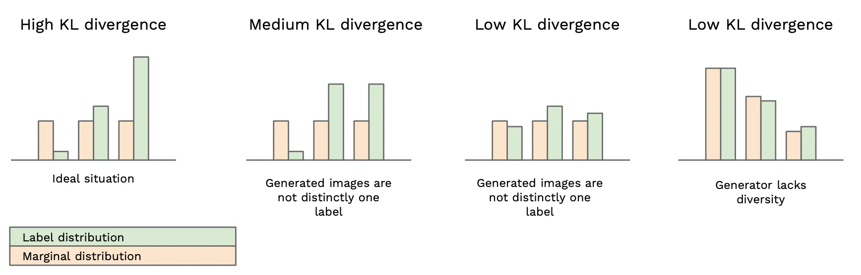
In summary, KL divergence is high when our distributions are dissimilar. That is, it is high when each generated image has a distinct label and the overall set of generated images has a diverse range of labels. Which is exactly how we defined it earlier :)
To get the final score, we take the exponential of the KL divergence (to make the score grow to bigger numbers to make it easier to see it improve) and finally take the average of this for all of our images. The result is the Inception score!
Written in mathematical terms
In mathematical parlance, the label distribution of an image is p(y|x), where y is the set of labels and x is the image. The marginal distribution is p(y). G(z) is the generated image, from ‘latent’ vector of random numbers z. This whole procedure looks like this in the original paper:


What are the limitations of the Inception Score?
Having a metric to optimize is a very important and powerful driver of research progress. The IS certainly has provided this for researchers. However, with any metric it’s important to know its limitations.
Here are a few considerations, for deeper analysis check out this paper.
- The score is limited by what the Inception (or other network) classifier can detect, which is directly linked to the training data (commonly ILSVRC 2014). This has a few repercussions:
- (1) If you’re learning to generate something not present in the classifier’s training data (e.g. sharks are not in ILSVRC 2014) then you may always get low IS despite generating high quality images since that image doesn’t get classified as a distinct class
- (2) If you’re generating images with a different set of labels from the classifier training set (say, you’re training the GAN to generate different varieties of poodles, or just elephants and ants) it can score lowly
- (3) If the classifier network cannot detect features relevant to your concept of image quality (e.g. there is evidence that CNNs rely heavily on local image textures for classification, and coarse shapes do not matter so much), then poor quality images may still get high scores. For example, you might generate people with two heads, but not get penalized for it.
- If your generator generates only one image per classifier image class, repeating each image many times, it can score highly (i.e. there is no measure of intra-class diversity)
- If your generator memorizes the training data and replicates it, it can score highly
In closing
Alright, I hope you found this useful! If there are things you’d like clarification on in this article, feel free to add a response or highlight.
If you’d like to learn more about machine learning, check out Octavian.AI.
Footnotes
- For a ceiling to the IS, imagine that our generators produce perfectly uniform marginal label distributions and a single label delta distribution for each image — then the score would be bounded by the number of labels.
- Technically, we’re finding the expectation value, or average of the distributions, since we sum them and divide by the total count so the resulting distribution’s values sum to give 1.0
- Marginal is a fancy way of saying we added everything together
- A probability distribution can be represented in many ways. Here in our network it’s a vector/list (same thing) of floating point values between 0.0 and 1.0, that sums to 1.0. Each entry in the vector implicitly represents the probability of a certain label. Somewhere else in our code will be a list of those labels.
- Note that if each image is indistinct (and has a uniform label distribution) then the marginal distribution is forced to be uniform.